computeGCBias (version 3.5.4+galaxy0)

BAM file:

Reference genome:

Using reference genome:

If your genome of interest is not listed, contact the Galaxy team

Effective genome size:

The effective genome size is the portion of the genome that is mappable. Large fractions of the genome are stretches of NNNN that should be discarded. Also, if repetitive regions were not included in the mapping of reads, the effective genome size needs to be adjusted accordingly. We provide a table of useful sizes here: http://deeptools.readthedocs.io/en/latest/content/feature/effectiveGenomeSize.html

Fragment length used for the sequencing:

If paired-end reads are used, the fragment length is computed from the BAM/CRAM file, so this is only needed for single-end data.

Region of the genome to limit the operation to:

This is useful when testing parameters to reduce the time required. The format is chr:start:end, for example "chr10" or "chr10:456700:891000".

Show advanced options:

GC bias plot:

If given, a diagnostic image summarizing the GC bias found on the sample will be created. (--plotFileFormat)

What it does

This tool computes the GC bias using the method proposed in Benjamini and Speed (2012) Nucleic Acids Res. (see below for further details). The output is used to plot the results and can also be used later on to correct the bias with the tool correctGCbias. There are two plots produced by the tool: a boxplot showing the absolute read numbers per GC-content bin and an x-y plot depicting the ratio of observed/expected reads per GC-content bin.

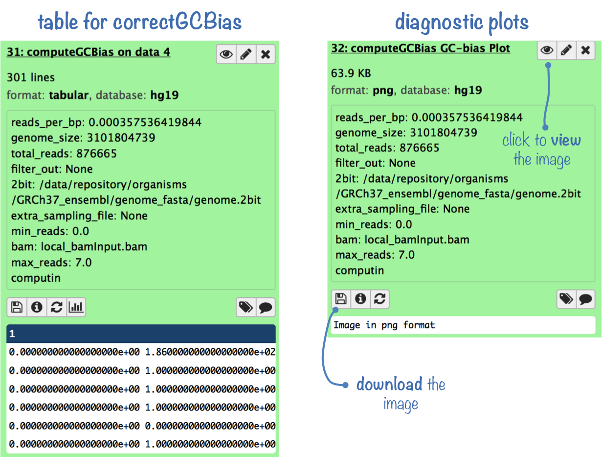
Output files

Diagnostic plots:
- box plot of absolute read numbers per GC-content bin
- x-y plot of observed/expected read ratios per GC-content bin
Tabular file: to be used for GC correction with correctGCbias

/repository/static/images/396f037a90638efc/computeGCBias_output.png

Theoretical Background

computeGCBias is based on a paper by Benjamini and Speed. The basic assumption of the GC bias diagnosis is that an ideal sample should show a uniform distribution of sequenced reads across the genome, i.e. all regions of the genome should have similar numbers of reads, regardless of their base-pair composition. In reality, the DNA polymerases used for PCR-based amplifications during the library preparation of the sequencing protocols prefer GC-rich regions. This will influence the outcome of the sequencing as there will be more reads for GC-rich regions just because of the DNA polymerase's preference.

computeGCbias will first calculate the expected GC profile by counting the number of DNA fragments of a fixed size per GC fraction where GC fraction is defined as the number of G's or C's in a genome region of a given length. The result is basically a histogram depicting the frequency of DNA fragments for each type of genome region with a GC fraction between 0 to 100 percent. This will be different for each reference genome, but is independent of the actual sequencing experiment.

The profile of the expected DNA fragment distribution is then compared to the observed GC profile, which is generated by counting the number of sequenced reads per GC fraction.

In an ideal experiment, the observed GC profile would, of course, look like the expected profile. This is indeed the case when applying computeGCBias to simulated reads.

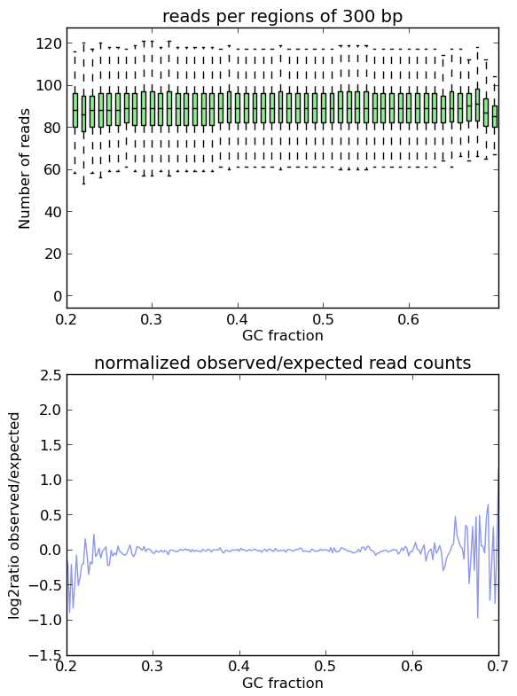
/repository/static/images/396f037a90638efc/GC_bias_simulated_reads_2L.png

As you can see, both plots based on simulated reads do not show enrichments or depletions for specific GC content bins, there is an almost flat line around the log2ratio of 0 (= ratio(observed/expected) of 1). The fluctuations on the ends of the x axis are due to the fact that only very, very few regions in the Drosophila genome have such extreme GC fractions so that the number of fragments that are picked up in the random sampling can vary.

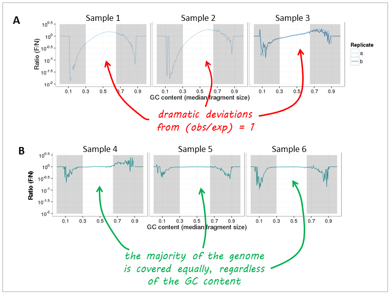
Now, let's have a look at real-life data from genomic DNA sequencing. Panels A and B can be clearly distinguished and the major change that took place between the experiments underlying the plots was that the samples in panel A were prepared with too many PCR cycles and a standard polymerase whereas the samples of panel B were subjected to very few rounds of amplification using a high fidelity DNA polymerase.

/repository/static/images/396f037a90638efc/QC_GCplots_input.png

Note: The expected GC profile depends on the reference genome as different organisms have very different GC contents. For example, one would expect more fragments with GC fractions between 30% to 60% in mouse samples (average GC content of the mouse genome: 45 %) than for genome fragments from, for example, Plasmodium falciparum (average genome GC content P. falciparum: 20%).

For more details, for example about when to exclude regions from the read distribution calculation, go here

For more information on the tools, please visit our help site.

For support or questions please post to Biostars. For bug reports and feature requests please open an issue on github.

This tool is developed by the Bioinformatics and Deep-Sequencing Unit at the Max Planck Institute for Immunobiology and Epigenetics.