Hi-C contact matrix correction
hicCorrectMatrix runs Imakaev's iterative correction, described in Imakaev et al. (2012), or Knight-Ruiz correction over a Hi-C matrix. For the matrix correction to be efficient, it is important to remove the unassembled scaffolds (e.g. NT_), mitochondrial DNA and Y chromosome and keep only full length chromosomes, as scaffolds create problems with matrix correction. Therefore we use the chromosome names (1-19, X, Y) here.
Important: Use ‘chr1 chr2 chr3 etc.’ if your genome index uses chromosome names with the ‘chr’ prefix.
Also, for the method to work correctly, bins with zero reads assigned to them should be removed as they can not be corrected. Also, bins with low number of reads should be removed, otherwise, during the correction step, the counts associated with those bins will be amplified (usually, zero and low coverage bins tend contain repetitive regions). Bins with extremely high number of reads can also be removed from the correction as they may represent copy number variations.
To aid in the identification of bins with low and high read coverage, the diagnostic plot function of hicCorrectMatrix must be used.
Indeed, hicCorrectMatrix works in two steps:
- Diagnostic plot: First a histogram containing the sum of contact per bin (row sum) is produced. This plot needs to be inspected to decide the best threshold for removing bins with lower number of reads.
- Correct: The second step removes the bins outside of the defined thresholds and perfroms the iterative correction.
Usage
This tool must be used on uncorrected matrices at restriction enzyme resolution or with merged bins (hicMergeMatrixBins).
Output
Diagnostic plot
The goal of the diagnostic plot is to help the user decide on a cutoff threshold that will ignore Hi-C matrix bins with few reads assigned to them. The plot is a histogram of the total number of Hi-C reads per matrix bin. A secondary scale based on the mean absolute deviation score, is shown on top of the figure. This secondary scale aims to offer 'normalized' values that are comparable across samples independently of the sequencing depth and the fraction of usable Hi-C reads. In all samples that we have studied, the histogram follows a bimodal distribution where the first peak is for bins with zero reads which usually occur at repetitive regions. Other low scoring bins tend to be close to repetitive regions. Also, low scoring bins can be caused by absence of a restriction site in the bin or because the restriction site is present but the restriction enzyme did not cut. The valley between the two peaks in the histogram is set by default as cutoff threshold. However, it is important to revise this as in some cases the selected value could not be correct.
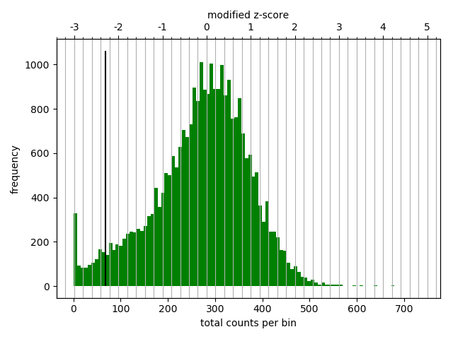
On the example plot above, a user can then use the lower threshold defined by the Median Absolute Deviation (MAD) method (black bold bar), or define its own threshold based on the contacts distribution.
Correct
Run the iterative correction and outputs the corrected matrix. This matrix can then be used with all downstream analysis tools such as hicPlotMatrix, pyGenomeTracks, hicPlotViewpoint, hicAggregateContacts for visualization of Hi-C data, hicCorrelate, hicPlotDistVsCounts, hicTransform, hicFindTADs, hicPCA for data and scores computation on Hi-C data.
It is noteworthy that hicSumMatrices and hicMergeMatrixBins must be performed on uncorrected matrices.